
Introduction
With today’s challenging economic times it has become more and more important to manage and rectify changing sales patterns and trends.
In today’s “get together” we shall be expanding our outlook by creating efficient and effective reports utilizing SQL Server Reporting Service 2016 and T-SQL, together with the DAX code that we created in our last “fire side chat”.
In order to make our reports more powerful and all-encompassing, in this chat, we shall be incorporating date and customer parameters to be utilized by our DAX code.
Thus, let’s get started.
Getting started
As our point of departure, we shall “pick up” with the Tabular project that we created in a previous “get together”. Should you not have had a chance to work through the discussion, do feel free to glance at the step by step discussion by clicking on the link below:
Beer and the tabular model DO go together
Management studio and our source code
Opening SQL Server 2016 Management Studio we shall once again have a look at the piece of DAX code that we utilized (see below).
The code seen above will be the code that we are going to incorporate into a standard T-SQL query and execute via a Linked Server! However, there I go again, getting ahead of myself!!
Creating the linked server
In order for us to work our ‘magic’, our first task is to create a linked server which may be utilized within the relational region of SQL Server and which points to our Tabular Analysis Server. The code may be seen below:

The code:
|
1 2 3 4 5 6 7 8 9 |
USE master GO EXEC sp_addlinkedserver @server='SQLShackTabularBeer2', -- local SQL name given to the linked server @srvproduct='', -- not used @provider='MSOLAP', -- OLE DB provider @datasrc='STR-SIMON\Steve2016tabular', -- analysis server name (machine name) @catalog='SQLShackTabularBeer1' -- default catalog/database |
Now that we have the code, the only thing left to do is to execute this code.
Now that our linked server has now created, we are ready to code our data extraction query.
Creating the query
Opening Management Studio from the relational side, we simply open a new query (see below)

We begin with our “Use” statement and point to our relational database. Having said this, the eagle-eyed reader will point out that we should be talking about DAX and the Tabular Model.
This is correct and we shall. The purpose of “USE” statement will become more apparent further in our discussion, thus for the meantime, let us just accept the statement.
We must declare a few variables. A notable one called @BeerStr, is defined as NVarchar(2000). This variable will contain our DAX query and through the usage of the linked server (that we created above) and the OpenQuery() struct, we shall perform our data extraction.
As a reminder, in the query that we discussed above, all of the parameters were hard-wired and whilst this is great for a demo, in real life scenarios, this not very useful.
We also declare three more variables (see below).
- @startt
- @endd
- @Customer
For our trials we shall set @startt to ‘201401’ i.e. January 2014, @endd to ‘201412’ i.e. December 2014 and @CustomerNo = 7 (The grocery firm Checker) which we have discussed in our past two “get togethers”.
Now here is the tricky part and we really need to discuss this prior to working with our code. Old Fortran programmers will tell you that should you want to place the name “O’Reilly” in a database field (with the apostrophe), then the raw data value must have TWO apostrophes.
Thus O’Reilly would look like O’’Reilly and THIS is where things become convoluted.
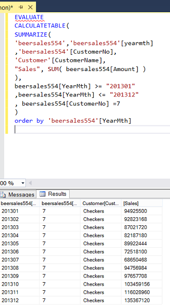
Our old code appeared similar to this
|
1 2 3 4 5 6 7 8 9 10 11 12 13 14 15 |
EVALUATE CALCULATETABLE( SUMMARIZE( 'beersales554','beersales554'[yearmth] ,'beersales554'[CustomerNo], 'Customer'[CustomerName], "Sales", SUM( beersales554[Amount] ) ), beersales554[YearMth] >= "201301" ,beersales554[YearMth] <= "201312" , beersales554[CustomerNo] =7 ) order by 'beersales554'[YearMth] |
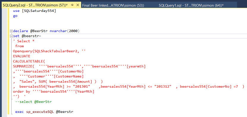
Our code for the new query is very different and may be seen below:

The code listing may be seen immediately below.
|
1 2 3 4 5 6 7 8 9 10 |
EVALUATE CALCULATETABLE( SUMMARIZE( ''''beersales554'''',''''beersales554''''[yearmth] ,''''beersales554''''[CustomerNo] , ''''Customer''''[CustomerName] , "Sales", SUM( beersales554[Amount] ) ) , beersales554[YearMth] >= "201301" ,beersales554[YearMth] <= "201312" , beersales554[CustomerNo] =7 ) order by ''''beersales554''''[YearMth] |
Building upon this we add a relational select statement and our OpenQuery function which may be seen below:

Our “Select” statement may be seen above. Do note that the DAX statement is “sandwiched” into a piece of T-SQL code.
As we want to be able to change the start and end dates and customer number dynamically from the reports that we are going to create, we do have a challenge. The challenge is that the dates and customer numbers cannot be placed directly into @startt, @endd and @customer and parsed at runtime. Should we attempt to do so and run the query, we shall encounter a runtime error. We need to circumvent this issue by first creating a text string with the parameters incorporated into the string.
We then execute this string utilizing sp_executeSQL, using the text string as the argument to the parameter.
|
1 2 3 |
exec sp_executeSQL @Beerstr |
Looking at the query first with hard-wired data we see the following:
Running the query we find the following.
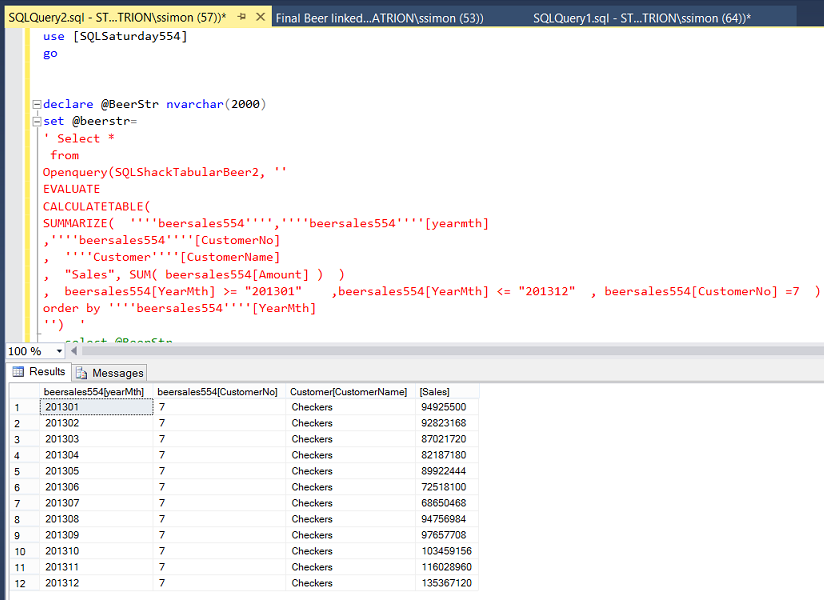
We note the results of the execution of the query and these results are similar to what we have seen in past “get togethers” so why go to all of this bother?
OK here is why!!! Many of us who work with MDX and DAX find that filtering and/or ensuring that query predicates function correctly is often very challenging.
Imagine if we could do a rough filter and then use T-SQL to do the final filtering. In short, we can do more complex filtering with T-SQL.
Alright, we are now at a point where we can make the final alterations to our query to permit it to be more flexible and to permit us to pass arguments to the query, dynamically at runtime.
We begin by removing the hard-wired dates and customer number and replacing these three “fields” with variables”. The changes to the code may be seen below:

We then run the query. The results may be seen below for ‘201401’ through ‘201412’ for Customer 7, “Checkers”.
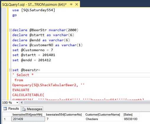
We note that there is only one record shown. This is correct.
Changing our dates to ‘201301’ through ‘201312’ we note data for the full year for “Checkers”.

Our final alteration to our query is to create a stored procedure (from the query), ensuring that we are able to pass arguments to our @startt, @endd, and @customerNo parameters.

Now that we have our final stored procedure, let us leave the “Hum Drum” work and create the report about which I was bragging.
Working in reporting services
In order to create our report, we open either Visual Studio 2015 or SQL Server Data Tools 2010 or greater. Should you have never worked with Reporting Services or should you not feel comfortable creating a Reporting Services project, then please do have a look at one of our earlier chats where the “creation” process is described in detail:
Beer and the tabular model DO go together
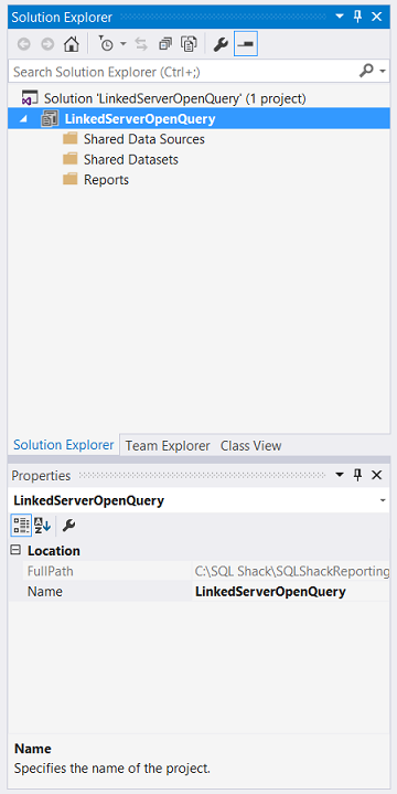
Having created a new Reporting Services Project (see above) we create a “Shared Data Source” called “OpenQuerry”. The data source points to the relational database where the stored procedure is hosted and that is why I set the SQLSaturday554 database within the “USE” statement, above.

Now that we have our data source all that is left to do is to add a new report.
Once again we right-click on the “Reports” folder and select “Add” and “New Item” (see below).

We add a new report as may be seen below:
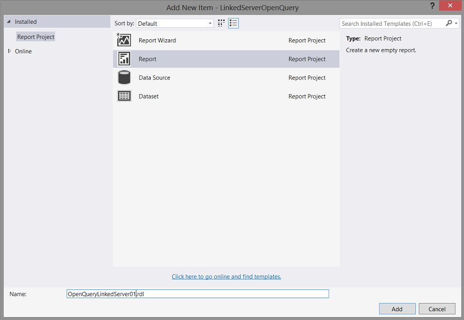
We then click “Add” and we find ourselves back on our drawing surface.

Creating the necessary datasets
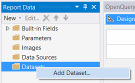
We right click upon the “Datasets” folder and select “Add Dataset” (see above).

Once again we create a new “Local Data Source” as described in the detail in the previous article. We click the “New” button (circled above) and create our local data source. We click “OK to continue.
We find ourselves back on the “Dataset Properties” window as may be seen below:

We choose a “Text” query and extract distinct Customer Numbers and Customer Names as may be seen above. We click “Refresh Fields” and then “OK” to continue.
Upon clicking “OK”, we find ourselves back on our drawing surface.

We note that the “Customer” Dataset has been created.
We repeat this process by creating “Start Date” and “End Date” datasets containing distinct year/month combinations.

The “Start Date” dataset code is shown above. We repeat the same task for the end date. Now, once again, the “wiseacres” amongst us will be saying “If these are date fields, why not utilize the same dataset for the start date and the end date”. Hold that thought as it will become clear within a few minutes.

Now that we have our three data sets , we are in a position to define our parameters that the end user will utilize for reporting .
Adding parameters to our new report
As a reminder, the stored procedure that we created above, accepts three arguments through the three respective parameters (see below). The arguments will be set (at runtime) within the report and then passed to the Stored Procedure.

We now shall create these three parameters within our SQL Server Reporting Services report.
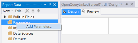
Right clicking upon the “Parameters” tab, we select “Add Parameter” (see above).

The “Report Parameter Properties” dialogue box is brought into view.
We call our first parameter start and leave the data type as text (see below).
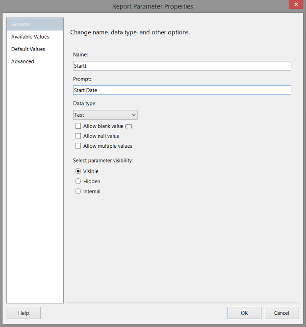
We now click upon the “Available Values” tab.

The “Report Parameter Properties” dialogue box opens (see above).
We select “Get Value from a query” (see above).

We select the “Start Date” dataset and set the “Value Field” to “YearMth” and the “Label Field” to “YearMth” as well. We click “OK to continue”. We find ourselves back on our Drawing Screen.
Creating the End Date parameter
The reader will recall that I had created an “End Date” data set as well.
This is the reason why.
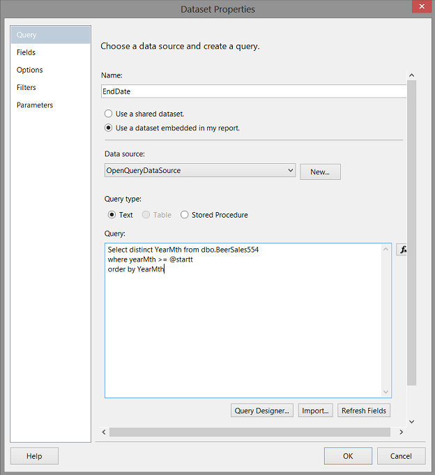
We re-open this data set, now that we have created the @startt parameter and change the query to include only “YearMth” values greater than or equal to the value that the user selected for the start date.
This will avoid queries being sent to the server, with a predicate such as
|
1 2 3 |
Where YearMth between ‘201312’ and ‘201301’ |
The modified dataset may be seen below:
Having reached this point, we are in a position to create the end date parameter pointing to the dataset shown above.
We then create the “Customer” parameter as shown below:

Creating our final dataset
The final dataset that we must create, will hold the data that is extracted from the Analysis Services Tabular database. For the sake of ease, we shall call this data set “Final Results”.

The result set for “FinalResults” will be obtained from the stored procedure that we created at the start of our “get together” (see above). Once again, we utilize the “OpenQueryDataSource” “Shared Data Source” and simply utilize the “execute” statement (see above).
We click “OK” to continue. We are brought back to our “Data Set” Properties window.
We click “Refresh Fields” to see the list of fields that the query will bring back to the report (see below).


We switch to the “Fields” tab as may be seen above.
“Houston, WE HAVE A PROBLEM!!!!!. The issue is that the “Select *” that we utilized in the stored procedure will not work. What we must use is a format similar to “Select CustomerNo, CustomerName…….” etc., instead of Select *.
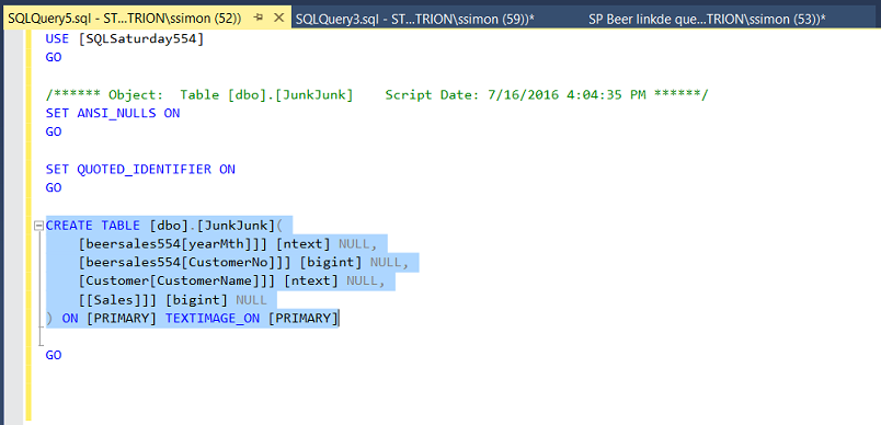
OK now the plot THICKENS!! The field names that are returned from the OpenQuery() are not what we would expect them to be. In order to determine what the actual field names are, we execute the Select statement into a table called junkjunk and from there determine the true field names.
The table structure of junkjunk may be seen below.
Now that we have the correct name of the fields, we go back into SQL Server Management Studio and change the stored procedure from:

To:

We reprocess our stored procedure.
Meanwhile back in Reporting Services, let us refresh our fields once again.

We note that our field names are now present.
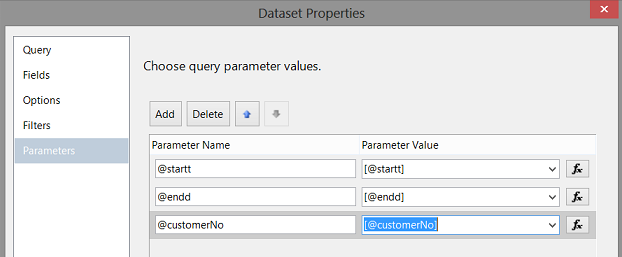
Our last task within this dataset is to set the “Parameters”.
We click on the Parameters tab (see below).
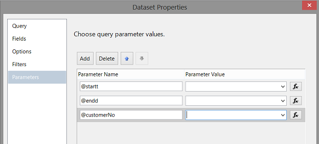
We note that our three parameters are present on the screen (see above).
All that we need do is to set the parameter values to those values selected by the end user. This is done as follows:

The end product looks as follows:
After clicking “OK” to this screen, we find ourselves back on our drawing surface (see below).

We note that the three parameters are present above our drawing surface, albeit greyed out.
Our next task is to add a “Chart” from the toolbox to our drawing surface. This chart will show the result set obtained from the database.
As we did in our last “get together”, we add a “column chart” to the drawing surface as shown below:

Our drawing surface looks as follows:

We resize the chart and allocate the “FinalResults” dataset to the “DataSetName” property of the chart (see highlighted below):

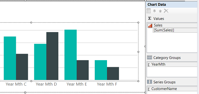
Setting the “Chart Data” properties
Our final task is to set the chart data properties in order for the chart axes to know what they should be displaying and where to display it. Our completed “Chart Data” window is shown below:
Let us give our query a test run
We click the preview button and the report surface changes. We are requested to enter in a “Start Date” (see below).

We shall choose ‘201303’ for a reason.
If our new “Enddate” dataset is functioning correctly then the first “end date” that we can select is either ‘201303’ or greater.
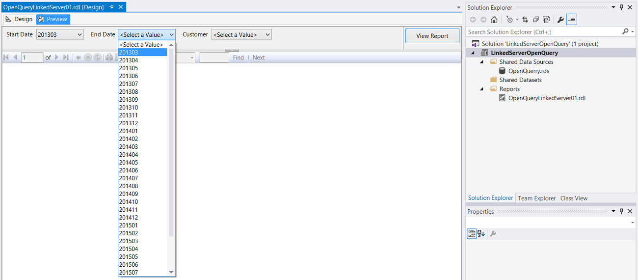
We note that this is in fact so (see above).
Setting the last of the arguments, the Customer parameter to “Checkers”, we obtain the following results when we click the view report button.
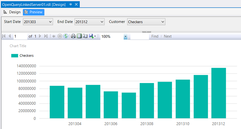
This is exactly what one would have expected to see.
Big Deal!! Why report in this fashion??
The answer is fairly simple. The big plus of utilizing your DAX code sandwiched in between two “slices” of T-SQL code, is that we may utilize T-SQL code within the predicate.
Let us say that we change the query slightly and move the customer number out of the DAX query and place it rather together within the T-SQL “Select” statement.
Doing so makes the query more versatile and we now have the option of viewing one customer at a time or viewing the results for all customers! (See the code below).

Further, let us say that when we wish to view the results from all customers, the way to achieve this is to pass -1 to the “CustomerNo” parameter. When we run the query, this is what we shall see.

On the other hand, should the incoming argument to the “CustomerNo” parameter not be -1 then the actual results for that “CustomerNo” will be displayed as may be seen below for “CustomerNo” 7.

Based upon what we originally constructed, in order to have this “one or all” facility, we must alter the code for our “CustomerNo” dataset. The necessary alterations may be seen below:
|
1 2 3 4 5 |
select distinct -1 as CustomerNo, 'All' as CustomerName from dbo.Customer union all Select distinct CustomerNO, CustomerName from dbo.Customer |
The modified data QUERY code may be seen in Addenda 2.
Conclusions
Once again we have come to the end of another “get together”.
Today we have seen how the DAX code that we have worked with in past “get togethers” may be utilized in combination with T-SQL. Somewhat as cold cuts may be sandwiched in between two slices of “T-SQL” bread. The advantages of doing so are that predicates can be more complex, albeit that we may be pulling more data from the tabular database that may be necessary. Thus it is a toss-up between efficiency and effectiveness.
Experimentation is key and I am sure that we shall find another interesting way to utilize what we have just been discussing.
Happy programming!
Addenda1
|
1 2 3 4 5 6 7 8 9 10 11 12 13 14 15 16 17 18 19 20 21 22 23 24 25 26 27 28 29 30 31 |
use [SQLSaturday554] go declare @BeerStr nvarchar(2000) declare @startt as varchar(6) declare @endd as varchar(6) declare @customerNO as varchar(1) set @Customerno = 7 set @startt = 201401 set @endd = 201412 set @beerstr= ' Select * from Openquery(SQLShackTabularBeer2, '' EVALUATE CALCULATETABLE( SUMMARIZE( ''''beersales554'''',''''beersales554''''[yearmth] ,''''beersales554''''[CustomerNo] , ''''Customer''''[CustomerName] , "Sales", SUM( beersales554[Amount] ) ) , beersales554[YearMth] >="' +@Startt + '",beersales554[YearMth] <="' +@endd + '", beersales554[CustomerNo] =' + @CustomerNO + ' ) order by ''''beersales554''''[YearMth] '') ' select @BeerStr exec sp_executeSQL @Beerstr |
Addenda 2
|
1 2 3 4 5 6 7 8 9 10 11 12 13 14 15 16 17 18 19 20 21 22 23 24 25 26 27 28 29 30 31 32 33 34 35 36 37 38 39 40 41 42 43 44 45 46 |
use [SQLSaturday554] go --Alter procedure FlexSQLShackQuery --( --@startt varchar(6), --@endd varchar(6), --@customerNo varchar(2) --) -- as declare @startt as varchar(6) declare @endd as varchar(6) set @startt = '201301' set @endd = '201312' declare @BeerStr nvarchar(2000) declare @startt1 as varchar(6) declare @endd1 as varchar(6) declare @customerNo1 as Varchar(2) declare @customerNO as varchar(2) set @Customerno = 7 set @startt1 = @startt set @endd1 = @endd Set @customerNo1 = @customerNo set @beerstr= ' Select [beersales554[yearMth]]] as YearMth , [beersales554[CustomerNo]]] as CustomerNo , [Customer[CustomerName]]] as CustomerName , [[Sales]]] as Sales from Openquery(SQLShackTabularBeer2, '' EVALUATE CALCULATETABLE( SUMMARIZE( ''''beersales554'''',''''beersales554''''[yearmth] ,''''beersales554''''[CustomerNo] , ''''Customer''''[CustomerName] , "Sales", SUM( beersales554[Amount] ) ) , beersales554[YearMth] >="' +@Startt1 + '",beersales554[YearMth] <="' +@endd1 + '") order by ''''beersales554''''[YearMth] '') where (1= (Case when ' + @CustomerNo1 +'= -1 then 1 else 2 end) OR ([beersales554[CustomerNo]]] = ' + @customerNo1 +')) ' --select @beerstr exec sp_executeSQL @Beerstr |
References:
- How to Create a Linked Server
- OPENQUERY (Transact-SQL)
- How to pass a variable to a linked server query
Steve has presented papers at 8 PASS Summits and one at PASS Europe 2009 and 2010. He has recently presented a Master Data Services presentation at the PASS Amsterdam Rally.
Steve has presented 5 papers at the Information Builders' Summits. He is a PASS regional mentor.
View all posts by Steve Simon
- Reporting in SQL Server – Using calculated Expressions within reports - December 19, 2016
- How to use Expressions within SQL Server Reporting Services to create efficient reports - December 9, 2016
- How to use SQL Server Data Quality Services to ensure the correct aggregation of data - November 9, 2016