To make the first steps into the BI world easier, you just need to build one SSAS Tabular model database. In this article, we will learn some basics of querying a SSAS Tabular model database with simple DAX queries, starting with a theoretical approach, and then retrieve data and analyze it.

Requirements for querying with DAX include SQL Server Management Studio 2014 or higher with an installed SSAS Tabular instance, and a deployed SSAS Tabular model database.

Preparing the environment

In order to get insight in a Tabular model database, the main method is data retrieval from tables through queries; after that, performing additional simple or complex calculations can take place.

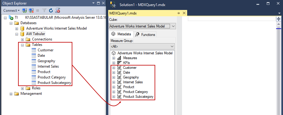
Querying a SSAS Tabular model database in this article will perform in SSMS, within the MDX query window, as shown in the picture:

Note: Don’t get confused with DAX code presence in a MDX query – both of them, DAX and MDX, can query a Tabular model database.

Data Analysis Expression (DAX) overview

DAX originally emerged from a Power Pivot add-in for Excel, as a formula language extension for creating calculated columns and measures for data analysis (which are also integral elements of one SSAS Tabular model database, too), but when Microsoft added support for DAX queries in SQL Server 2012, BI experts started “daxing” data from Tabular model databases.

That trend continues, because of simplicity and fast query execution (related to DirectQuery mode in SSAS Tabular).

DAX query consists of a function and number of expressions (e.g.):

Functions are the main part of the query, and they act similar to some T-SQL statements (as we will see later). Expressions consist of values, operators and constants. The difference between expressions in Excel (Power Pivot) and SSMS should be apparent; In Power PIvot, expressions start with equal sign “=”, and they look like formulas:

In this example, ‘Product’[Standard Cost] is value, and there are no operators (+, – e.g.) or constants.

DAX expressions in SSMS are more complex, because of the whole syntax. Although there are many rules, the following are just some examples.

Querying SSAS Tabular model database

The foundation of every Tabular DAX query is the Evaluate statement:

Or displayed in SSMS, a query result below:

The Evaluate statement is similar to a SELECT in T-SQL, because it retrieves all columns from a particular table, in this case, the Product table. Similar T-SQL code would be:

The query result, the selected columns, would be the same as in querying the SQL Server database, but the main difference is the naming of columns. Columns in SSAS Tabular model database don’t use CamelCase or pascalCase naming methods. They include the actual table name in the title and allow space characters, as shown in the picture below:

It is important to know the exact names of the elements, because of using particular tables and columns in DAX expression(s). Regarding the syntax, format tables like this:

Now, the table Product in this expression is surrounded with apostrophe characters, and executing the query shows the same result, as with ‘Product’ expression without apostrophes.

Note: Statements in DAX query code are case-insensitive:

To start creating some complex queries, format the evaluate statement as shown:

evaluate ( ‘Product’ )

or like this, which will be used in the article:

Putting brackets (as parenthesis operator) after function means that query will become complex, although this query shows the same results as in the previous queries. Also, choose a suitable format according to your personal preferences, but pay attention on the examples from this article (number of brackets etc.).

1. VALUES function

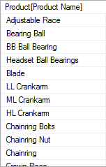
   This query will show all values of the Product Name column only:

   1 2 3

   evaluate(values('Product'[Product Name]))

   Values function shows the distinct values of specified column, without duplicates:

   

2. ORDER BY function

   ORDER BY function is exact as it is in T-SQL:

   1 2 3 4

   evaluate('Product') order by [Product Subcategory Id]

   It orders the query result according to the selected column as a parameter. In this case, the parameter is Product Subcategory Id.

   Multiple columns can be set as parameters, as shown:

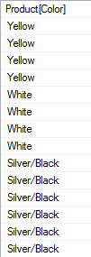
   1 2 3 4

   evaluate('Product') order by [Product Subcategory Id], [Color]

   

   Order can be ascending or descending (ASC or DESC in the end of statement):

   1 2 3 4

   evaluate('Product') order by [Color] DESC

   

3. START AT function

   This function sets the starting point (first row) from which values will be displayed:

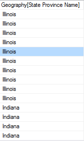
   1 2 3 4 5

   evaluate('Geography') order by [State Province Name] start at "Illinois"

   In this example, the value “Illinois” is set:

   

4. FILTER function

   With FILTER function, particular column values with distinctive rows can be isolated as in T-SQL WHERE statement:

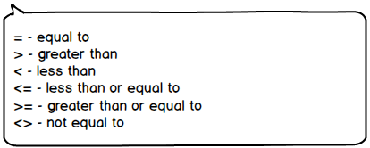
   1 2 3

   evaluate(filter('Geography', [State Province Name] = "North Carolina"))

   

   In this statement, use the comparison operators:

   

   One more example of the Filter function, with a numeric value:

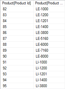
   1 2 3

   evaluate(filter('Product', [Product Id] >= 82))

   

   Notice that the value 82 doesn’t have any surrounding symbols, and “North Carolina” has quotation marks – that is because of the data type of the columns (Int and Text).

5. ADDCOLUMN function

   This is function adds a custom column Daily Profit, and it is dependent on the FILTER function:

   1 2 3 4 5 6 7 8

   evaluate (filter(addcolumns( 'Product', "Daily Profit", 'Product'[List Price] - 'Product'[Standard Cost]), 'Product'[List Price] > 1)) order by 'Product'[Product Subcategory Id]

   As can be seen, column Daily Profit is the product of calculation (subtraction) between two previously specified columns.

   

6. SUMMARIZE function

   This function acts as an aggregated and simplified substitute of T-SQL GROUP BY or JOIN statements in T-SQL. In one case, the desired columns are retrieved and shown as a result of the query, without any mathematical operation:

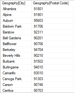
   1 2 3 4

   evaluate summarize('Geography', 'Geography'[City], 'Geography'[Postal Code])

   

   The syntax for the SUMMARIZE function is to define the primary table (Product), then define the columns which will be included in the result.

   Also, with the Order by clause included:

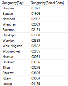
   1 2 3 4 5

   evaluate summarize('Geography', 'Geography'[City], 'Geography'[Postal Code]) order by [Postal Code]

   The result is put in order of Postal code:

   

   In this example we will include summary calculations of Total Days of Manufacture August 2016:

   1 2 3 4 5

   evaluate summarize('Product', "Total Days of Manufacture August 2016", sum('Product'[Days To Manufacture]))

   

   This result was created by defining the primary table, and then naming the measure (the title must be within quotation marks) and performing the calculation with a SUM function on the particular column with the table specified.

7. ROW function

   These statements can be very interesting to show a combination of particular functions while querying a SSAS Tabular model database.

   The ROW function returns a single, custom titled column and one row with the specific value. Execute these specific (and interesting) expressions:

   • Show the current date and time with NOW():

     1 2 3

     evaluate(ROW("Current date and time", Now()))

   • Show the PI number with PI():

     1 2 3

     evaluate(ROW("The PI Number", PI()))

   • Convert degrees to radians with DEGREES function:

     1 2 3

     evaluate(ROW("Degrees to Radians", DEGREES(90)))

   • Calculate the average value of particular column with AVERAGE function:

     1 2 3

     evaluate(ROW("Average Price", AVERAGE('Product'[List Price])))

   Quick tip: Try other aggregate functions like MAX, MIN or COUNT instead of AVERAGE, and don’t forget to rename the column properly

   • Retrieve the position of specified letter in particular word with SEARCH function:

     1 2 3

     evaluate(ROW("Position of letter B", SEARCH("b", "Tabular")))

   • We can even perform some basic mathematical operations within the query, and also add some more complex functions:

     1 2 3

     evaluate(ROW("Calculator", 25*6-6))

   I hope you have enjoyed these examples and querying your SSAS Tabular model database!

   Useful links

   • Data Analysis Expressions (DAX) Overview
   • DAX Syntax Reference
   • Tabular Models (SSAS)
   
   
   • Author
   • Recent Posts

   

   Daniel Tikvicki

   Daniel is a librarian who ran into a vortex of IT world, where he is levitating and learning constantly. He likes books, merely all forms of artistic expression (being a musician/poet himself), and he is underground publisher (fanzines and experimental music). Also, the points of interest include theology, mythology and pseudoscience.
   
   Daniel is currently working for ApexSQL LLC as Software sales engineer where he specializes for the BI environment.

   

   Latest posts by Daniel Tikvicki (see all)

   • How to monitor the SQL Server tempdb database - July 6, 2017
   • How to monitor total SQL Server indexes size - June 12, 2017
   • How to set and use encrypted SQL Server connections - May 8, 2017

   Related posts:

   1. How to query a SSAS Tabular model database with MDX expressions
   2. Time Intelligence in Analysis Services (SSAS) Tabular Models
   3. Creating your first SSAS tabular model database
   4. How to create a simple SSRS Report using a SSAS Tabular model database
   5. How to automate SSAS tabular model processing in SQL Server 2016