This post opens a series of blog posts dedicated to my observations of the new cardinality estimator in SQL Server 2014. But, before we jump to the new features, I’d like to provide some background, to make the next posts clearer.
We’ll start by discussing the role of Cardinality Estimation in SQL Server, trying to answer – what is it and why it is needed.
SQL Server has the Cost Based Optimizer. The optimizer chooses the cheapest plan, where cost represents an estimate of the resource consumption.
Cardinality estimation is the crucial mechanism in SQL Server, because, it is a main argument in the costing function. Cardinality estimation influences a lot of things, here are some of them:
- Access Method Strategy
- Join Order Choise
- Join Type Choise
- Memory grants
- Optimization Efforts Spent
- Whole Plan Shape
A lot of things are not included in this general list, however, they are also influenced by cardinality.
Let’s create a simple synthetic database “opt”, it will be used in this and future blog posts for the simple demos. It contains three plain tables of 1000 rows each with primary keys, two of them have a foreign key relationship.
|
1 2 3 4 5 6 7 8 9 10 11 12 13 14 15 16 17 18 19 20 21 22 23 |
use master; go if db_id('opt') is not null drop database opt; go create database opt; go use opt; go create table t1(a int not null, b int not null, c int check (c between 1 and 50), constraint pk_a primary key(a)); create table t2(b int not null, c int, d char(10), constraint pk_b primary key(b)); create table t3(c int not null, constraint pk_c primary key(c)); go insert into t1(a,b,c) select number, number%100+1, number%50+1 from master..spt_values where type = 'p' and number between 1 and 1000; insert into t2(b,c) select number, number%100+1 from master..spt_values where type = 'p' and number between 1 and 1000; insert into t3(c) select number from master..spt_values where type = 'p' and number between 1 and 1000; go alter table t1 add constraint fk_t2_b foreign key (b) references t2(b); go create statistics s_b on t1(b); create statistics s_c on t1(c); create statistics s_c on t2(c); create statistics s_d on t2(c); go |
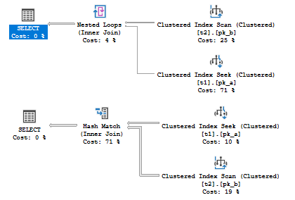
Now, imagine simple queries that joins two tables and filter rows.
|
1 2 3 4 5 6 7 |
set showplan_xml on go select * from t1 join t2 on t1.a = t2.c where t1.a <= 10 select * from t1 join t2 on t1.a = t2.c where t1.a <= 100 go set showplan_xml off go |
Depending on the estimated number of rows (estimated cardinality), we get different plans, even in such a simple case!

The only thing that is different, is the estimated number of rows. These different estimates lead to, at least, three item changes, according to the list mentioned above:
- Access Method Strategy (t2 Seek vs. t2 Scan)
- Join Order Choise (t1 Join t2 vs. t2 Join t1)
- Join Type Choise (Nested Loops Join vs. Merge Join)
Now we may see, how sensitive is the Query Optimizer to the cardinality estimation. Wrong estimates may lead to a very inefficient plan, that’s why it is so important component of SQL Server, and that’s why I think it is worth to spend time learning how these estimates are made.
Next we’ll discuss a place of Cardinality Estimation in the whole optimization process.
Table of Contents
References
- Cardinality Estimation (SQL Server)
- Troubleshooting Poor Query Performance: Cardinality Estimation
- Query Tuning Fundamentals: Density, Predicates, Selectivity, and Cardinality
See more
Check out ApexSQL Plan, to view SQL execution plans, including comparing plans, stored procedure performance profiling, missing index details, lazy profiling, wait times, plan execution history and more

- SQL Server 2017: Adaptive Join Internals - April 30, 2018
- SQL Server 2017: How to Get a Parallel Plan - April 28, 2018
- SQL Server 2017: Statistics to Compile a Query Plan - April 28, 2018


